Pre-ACCESS CMIP5/MODIS analysis scripts
The fifth phase of the Coupled Model Intercomparison Project (CMIP5) provides a multi-model
framework for comparing the mechanisms and responses of climate models from around the world.
However, the workload of retrieving a certain climate statistic from all these models, each of which includes
several ensemble members, is tremendous. Not only that, it is too
often a repetitive process which impedes new research and
hypothesis testing.
Our NASA ACCESS project is designed to simplify and accelerate this
process.
To begin, we have documented below a prototypical example of CMIP5
analysis and evaluation using traditional NCO commands on
netCDF3-format model and HDF-EOS format observational (NASA
MODIS satellite instrument) datasets.
These examples complement the NCO User's Guide by detailing
in-depth data analysis in a frequently encountered “real
world” context.
Graphical representations of the results (NCL scripts available upon
request) are provided to illustrate physical meaning of the analysis.
Over the summer of 2013, we will add scripts which make use of new NCO
features that combine all the loops in the analysis into single
commands by exploiting NCO's new group aggregation and
arithmetic features.
Sample Scripts
- Combine Files
Sometimes, the data of one ensemble member will be stored in several files to
reduce single file size. This script illustrates how to concatenate these files into one,
including:
- Obtain the number and names (or partial names) of files in directory;
- Concatenate files along record dimension (the left-most dimension) using ncrcat.
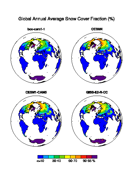
- Global Distribution of Long-term Average (see Fig. 1)
- Average the ensemble members of each model using ncea;
- Average along the record dimension (the left-most) using ncra;
- Store the results of one model as a group in the output file using ncecat with the
option of –gag;
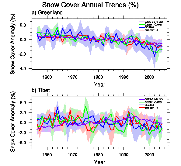
- Annual Average over Regions (see Fig. 2)
- Spatial average using ncap2 and ncwa;
- Change the order of dimensions using ncpdq;
- Annual average using ncra;
- Anomaly from long-term average using ncbo;
- Standard deviation using ncbo and ncea;
- Rename variables using ncrename;
- Edit attributions using ncatted;
- Linear regression using ncap2;
- Use ncap2 with commands file (i.e., .nco file);
- Move variables around using ncks.
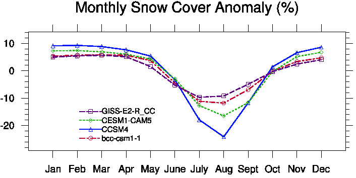
- Monthly Cycle (see Fig. 3)
- Anomaly from annual-average
- Regrid MODIS Data
- Regrid using bilinear interpolation;
- Rename variables, dimensions and attributions using ncrename.
- Add Coordinates to MODIS Data
- Permute MODIS Coordinates
The latitude of MODIS data is from 90oN to -90oN, and the longitude is from -180oE to
180oE. However, CMIP5 is from -90oN to 90oN, and from 0oE to 360oE. So this script
illustrates how to change MODIS coordinate to that of CMIP5.
 |
|
|
| Fig. 1 Global Distribution of Long-term Average. |
Fig. 2 Annual Average over Regions. |
Fig. 3 Monthly Cycle. |
1 Combine Files
#!/bin/bash ## shell type
shopt -s extglob ## enable extended globbing
##===========================================================================
## Some of the models cut one ensemble member into several files, which include data of different time periods.
## We’d better concatenate them into one at the beginning so that we won’t have to think about which files we need if we want to retrieve a specific time period later.
##
## Method:
## - Make sure ’time’ is the record dimension (i.e., left-most)
## - ncrcat
##===========================================================================
drc_in=’/home/wenshanw/data/cmip5/’## directory of input files
var=( ’snc’ ’snd’ ) ## variables
rlm=’LImon’## realm
xpt=( ’historical’ ) ## experiment ( could be more )
for var_id in {0..1}; do ## loop over two variables
## names of all the models (ls [get file names]; cut [get the part for model names]; sort; uniq [remove duplicates]; awk [print])
mdl_set=$( ls ${drc_in}${var[var_id]}_${rlm}_*_${xpt[0]}_*.nc | cut -d ’_’ -f 3 | sort | uniq -c | awk ’{print $2}’ )
## number of models (echo [print contents]; wc [count])
mdl_nbr=$( echo ${mdl_set} | wc -w )
echo "=============================="
echo "There are" ${mdl_nbr} "models for" ${var[var_id]}.
for mdl in ${mdl_set}; do ## loop over models
## names of all the ensemble members
nsm_set=$( ls ${drc_in}${var[var_id]}_${rlm}_${mdl}_${xpt[0]}_*.nc | cut -d ’_’ -f 5 | sort | uniq -c | awk ’{print $2}’ )
nsm_nbr=$( echo ${nsm_set} | wc -w )
## number of ensemble members in each model
echo "------------------------------"
echo "Model" ${mdl} "includes" ${nsm_nbr} "ensemble member(s):"
echo ${nsm_set}"."
for nsm in ${nsm_set}; do ## loop over ensemble members
fl_nbr=$( ls ${drc_in}${var[var_id]}_${rlm}_${mdl}_${xpt[0]}_${nsm}_*.nc | wc -w ) ## number of files in this ensemble member
if [ ${fl_nbr} -le 1 ]
## if there is only 1 file, continue to next loop
then
echo "There is only 1 file in" ${nsm}.
continue
fi
echo "There are" ${fl_nbr} "files in" ${nsm}.
## starting date of data (sed [the name of the first file includes the starting date])
yyyymm_str=$( ls ${drc_in}${var[var_id]}_${rlm}_${mdl}_${xpt[0]}_${nsm}_*.nc | sed -n ’1p’ | cut -d ’_’ -f 6 | cut -d ’-’ -f 1 )
## ending date of data (sed [the name of the last file includes the ending date])
yyyymm_end=$( ls ${drc_in}${var[var_id]}_${rlm}_${mdl}_${xpt[0]}_${nsm}_*.nc | sed -n "${fl_nbr}p" | cut -d ’_’ -f 6 | cut -d ’-’ -f 2 )
## concatenate the files of one ensemble member into one along the record dimension (now is time)
ncrcat -O ${drc_in}${var[var_id]}_${rlm}_${mdl}_${xpt[0]}_${nsm}_*.nc ${drc_in}${var[var_id]}_${rlm}_${mdl}_${xpt[0]}_${nsm}_${yyyymm_str}-${yyyymm_end}
## remove useless files
rm ${drc_in}${var[var_id]}_${rlm}_${mdl}_${xpt[0]}_${nsm}_!(${yyyymm_str}-${yyyymm_end})
done
done
done
2 Global Distribution of Long-term Average
#!/bin/bash
##===========================================================================
## After one-ensemble-one-file.sh
## Example: Long-term average of each model globally
##===========================================================================
##---------------------------------------------------------------------------
## parameters
drc_in=’/home/wenshanw/data/cmip5/’## directory of input files
drc_out=’/home/wenshanw/data/cmip5/output/’## directory of output files
var=( ’snc’ ’snd’ ) ## variables
rlm=’LImon’## realm
xpt=( ’historical’ ) ## experiment ( could be more )
fld_out=( ’snc/’ ’snd/’ ) ## folders of output files
##---------------------------------------------------------------------------
for var_id in {0..1}; do ## loop over two variables
## names of all models (ls [get file names]; cut [get the part for model names]; sort; uniq [remove duplicates]; awk [print])
mdl_set=$( ls ${drc_in}${var[var_id]}_${rlm}_*_${xpt[0]}_*.nc | cut -d ’_’ -f 3 | sort | uniq -c | awk ’{print $2}’ )
mdl_num=$( echo ${mdl_set} | wc -w )
## number of models (echo [print contents]; wc [count])
for mdl in ${mdl_set}; do ## loop over models
## average all the ensemble members of each model
ncea -O -4 -d time,"1956-01-01 00:00:0.0","2005-12-31 23:59:9.9" ${drc_in}${var[var_id]}_${rlm}_${mdl}_${xpt[0]}_*.nc ${drc_out}${fld_out[var_id]}${var[var_id]}_${rlm}_${mdl}_${xpt[0]}_all-nsm_195601-200512.nc
## average along time
ncra -O ${drc_out}${fld_out[var_id]}${var[var_id]}_${rlm}_${mdl}_${xpt[0]}_all-nsm_195601-200512.nc ${drc_out}${fld_out[var_id]}${var[var_id]}_${mdl}.nc
echo Model ${mdl} done!
done
## Remove temporary files to avoid file name confliction
rm ${drc_out}${fld_out[var_id]}${var[var_id]}*historical*.nc
## Store models as groups in the output file
ncecat -O --gag ${drc_out}${fld_out[var_id]}${var[var_id]}_*.nc ${drc_out}${fld_out[var_id]}${var[var_id]}_${rlm}_all-mdl_${xpt[0]}_all-nsm_clm.nc
echo Var ${var[var_id]} done!
done
3 Annual Average over Regions
#!/bin/bash
# includes gsl_rgr.nco
##===========================================================================
## After one-ensemble-one-file.sh
## Example: Annual trend of each model over Greenland and Tibet ( time- and spatial-average, standard deviation, anomaly and linear regression)
##===========================================================================
##---------------------------------------------------------------------------
## parameters
drc_in=’/home/wenshanw/data/cmip5/’## directory of input files
drc_out=’/home/wenshanw/data/cmip5/output/’## directory of output files
var=( ’snc’ ’snd’ ) ## variables
rlm=’LImon’## realm
xpt=( ’historical’ ) ## experiment ( could be more )
fld_out=( ’snc/’ ’snd/’ ) ## folders of output files
##------------------------------------------------------------
for var_id in {0..1}; do ## loop over two variables
## names of all models (ls [get file names]; cut [get the part for model names]; sort; uniq [remove duplicates]; awk [print])
mdl_set=$( ls ${drc_in}${var[var_id]}_${rlm}_*_${xpt[0]}_*.nc | cut -d ’_’ -f 3 | sort | uniq -c | awk ’{print $2}’ )
for mdl in ${mdl_set}; do ## loop over models
for fn in $( ls ${drc_in}${var[var_id]}_${rlm}_${mdl}_${xpt[0]}_*.nc ); do
## loop over ensemble members
pfx=$( echo ${fn} | cut -d’/’ -f6 | cut -d’_’ -f1-5 )
## part of the file name
## retrieve the 2 zones
## calculate the geographical weight first
ncap2 -O -s ’gw = cos(lat*3.1415926/180.); gw@long_name="geographical weight";gw@units="ratio"’ ${fn} ${drc_out}${fld_out[var_id]}${pfx}_gw.nc
## Greenland
ncwa -O -w gw -d lat,60.0,75.0 -d lon,300.0,340.0 -a lat,lon ${drc_out}${fld_out[var_id]}${pfx}_gw.nc ${drc_out}${fld_out[var_id]}${pfx}_gw_1.nc
## Tibet
ncwa -O -w gw -d lat,30.0,40.0 -d lon,80.0,100.0 -a lat,lon ${drc_out}${fld_out[var_id]}${pfx}_gw.nc ${drc_out}${fld_out[var_id]}${pfx}_gw_2.nc
## concatenate 2 zones together
ncecat -O -u zone ${drc_out}${fld_out[var_id]}${pfx}_gw_?.nc ${drc_out}${fld_out[var_id]}${pfx}_gw_zone4.nc
## change the order of the dimension so that the record dimension is ’time’
ncpdq -O -a time,zone ${drc_out}${fld_out[var_id]}${pfx}_gw_zone4.nc ${drc_out}${fld_out[var_id]}${pfx}_gw_zone4.nc
## remove the temporary files (optional)
rm ${drc_out}${fld_out[var_id]}${pfx}_gw_?.nc ${drc_out}${fld_out[var_id]}${pfx}_gw.nc
## annual average (use the feature of ’Duration’)
ncra -O --mro -d time,"1956-01-01 00:00:0.0","2005-12-31 23:59:9.9",12,12 ${drc_out}${fld_out[var_id]}${pfx}_gw_zone4.nc ${drc_out}${fld_out[var_id]}${pfx}_yrly.nc
## anomaly
## long-term average
ncwa -O -a time ${drc_out}${fld_out[var_id]}${pfx}_yrly.nc ${drc_out}${fld_out[var_id]}${pfx}_clm.nc
## subtract long-term average
ncbo -O --op_typ=- ${drc_out}${fld_out[var_id]}${pfx}_yrly.nc ${drc_out}${fld_out[var_id]}${pfx}_clm.nc ${drc_out}${fld_out[var_id]}${pfx}_anm.nc
done
rm ${drc_out}${fld_out[var_id]}${var[var_id]}_${rlm}_${mdl}_${xpt[0]}_*_yrly.nc
## average over all the ensemble members
ncea -O -4 ${drc_out}${fld_out[var_id]}${var[var_id]}_${rlm}_${mdl}_${xpt[0]}_*_anm.nc ${drc_out}${fld_out[var_id]}${var[var_id]}_${rlm}_${mdl}_${xpt[0]}_all-nsm_anm.nc
## standard deviation ------------------------------
for fn in $( ls ${drc_out}${fld_out[var_id]}${var[var_id]}_${rlm}_${mdl}_${xpt[0]}_*_anm.nc ); do
pfx=$( echo ${fn} | cut -d’/’ -f8 | cut -d’_’ -f1-5 )
## difference between each ensemble member and the average of all members
ncbo -O --op_typ=- ${fn} ${drc_out}${fld_out[var_id]}${var[var_id]}_${rlm}_${mdl}_${xpt[0]}_all-nsm_anm.nc ${drc_out}${fld_out[var_id]}${pfx}_dlt.nc
done
## RMS
ncea -O -y rmssdn ${drc_out}${fld_out[var_id]}${var[var_id]}_${rlm}_${mdl}_${xpt[0]}_*_dlt.nc ${drc_out}${fld_out[var_id]}${var[var_id]}_${rlm}_${mdl}_${xpt[0]}_all-nsm_sdv.nc
## rename variables
ncrename -v ${var[var_id]},sdv ${drc_out}${fld_out[var_id]}${var[var_id]}_${rlm}_${mdl}_${xpt[0]}_all-nsm_sdv.nc
## edit attributions
ncatted -a standard_name,sdv,a,c,"_standard_deviation_over_ensemble" -a long_name,sdv,a,c," Standard Deviation over Ensemble" -a original_name,sdv,a,c," sdv" ${drc_out}${fld_out[var_id]}${var[var_id]}_${rlm}_${mdl}_${xpt[0]}_all-nsm_sdv.nc
##------------------------------------------------------------
## linear regression -----------------------------------------
##!!!!!!!!!!!!!!!!!!!!!!!!!!!!!!!!!!!!!!!!!!!!!!!!!!!!!!!!!!!!!!!!!!!!!!!!!!!
## have to change the name of variable in the commands file of gsl_rgr.nco manually (gsl_rgr.nco is listed below)
ncap2 -O -S gsl_rgr.nco ${drc_out}${fld_out[var_id]}${var[var_id]}_${rlm}_${mdl}_${xpt[0]}_all-nsm_anm.nc ${drc_out}${fld_out[var_id]}${var[var_id]}_${rlm}_${mdl}_${xpt[0]}_all-nsm_anm_rgr.nc
##!!!!!!!!!!!!!!!!!!!!!!!!!!!!!!!!!!!!!!!!!!!!!!!!!!!!!!!!!!!!!!!!!!!!!!!!!!!
## get rid of temporary variables
ncks -O -v c0,c1,pval,${var[var_id]},gw ${drc_out}${fld_out[var_id]}${var[var_id]}_${rlm}_${mdl}_${xpt[0]}_all-nsm_anm_rgr.nc ${drc_out}${fld_out[var_id]}${var[var_id]}_${mdl}.nc
##------------------------------------------------------------
## move the variable ’sdv’ into the anomaly files (i.e., *anm.nc files)
ncks -A -v sdv ${drc_out}${fld_out[var_id]}${var[var_id]}_${rlm}_${mdl}_${xpt[0]}_all-nsm_sdv.nc ${drc_out}${fld_out[var_id]}${var[var_id]}_${mdl}.nc
rm ${drc_out}${fld_out[var_id]}${var[var_id]}_*historical*
echo Model ${mdl} done!
done
## Store models as groups in the output file
ncecat -O --gag ${drc_out}${fld_out[var_id]}${var[var_id]}_*.nc ${drc_out}${fld_out[var_id]}${var[var_id]}_${rlm}_all-mdl_${xpt[0]}_all-nsm_annual.nc
echo Var ${var[var_id]} done!
done
//linear regression
//Caution: make sure the variable name is in agreement with the main script (now is ’snd’)
//declare variables
*c0[$zone]=0.; //intercept
*c1[$zone]=0.; //slope
*sdv[$zone]=0.; //standard deviation
*covxy[$zone]=0.; //covariance
*x = double(time);
for (*zone_id=0;zone_id<$zone.size;zone_id++) //loop over zones
{
gsl_fit_linear(time,1,snd(:,zone_id),1,$time.size, &tc0, &tc1, &cov00, &cov01,&cov11,&sumsq); //linear regression function
c0(zone_id) = tc0; //store the results
c1(zone_id) = tc1;
covxy(zone_id) = gsl_stats_covariance(time,1,$time.size,double(snd(:,zone_id)),1,$time.size); //covariance function
sdv(zone_id) = gsl_stats_sd(snd(:,zone_id), 1, $time.size); //standard deviation function
}
//pval------------------------------------------------------------
*time_sdv = gsl_stats_sd(time, 1, $time.size);
*r_value = covxy/(time_sdv*sdv);
*t_value = r_value/sqrt((1-r_value^2)/($time.size-2));
pval = abs(gsl_cdf_tdist_P(t_value, $time.size-2) - gsl_cdf_tdist_P(-t_value, $time.size-2));
//----------------------------------------------------------------
//write RAM variables to disk
//------------------------------------------------------------
//usually NCO writes the outputs directly to disk
//inside .nco files, using RAM variables, declared by *, will shorten running time
//write the final outputs using ram_write()
//------------------------------------------------------------
ram_write(c0);
ram_write(c1);
4 Monthly Cycle
#!/bin/bash
##============================================================
## After one-ensemble-one-file.sh
## Example: Monthly cycle of each model in Greenland
##============================================================
##------------------------------------------------------------
## parameters
drc_in=’/home/wenshanw/data/cmip5/’## directory of input files
drc_out=’/home/wenshanw/data/cmip5/output/’## directory of output files
var=( ’snc’ ’snd’ ) ## variables
rlm=’LImon’## realm
xpt=( ’historical’ ) ## experiment ( could be more )
fld_out=( ’snc/’ ’snd/’ ) ## folders of output files
##------------------------------------------------------------
for var_id in {0..1}; do ## loop over two variables
## names of all models (ls [get file names]; cut [get the part for model names]; sort; uniq [remove duplicates]; awk [print])
mdl_set=$( ls ${drc_in}${var[var_id]}_${rlm}_*_${xpt[0]}_*.nc | cut -d ’_’ -f 3 | sort | uniq -c | awk ’{print $2}’ )
for mdl in ${mdl_set}; do ## loop over models
## average all the ensemble members in each model
ncea -O -4 -d time,"1956-01-01 00:00:0.0","2005-12-31 23:59:9.9" ${drc_in}${var[var_id]}_${rlm}_${mdl}_${xpt[0]}_*.nc ${drc_out}${fld_out[var_id]}${var[var_id]}_${rlm}_${mdl}_${xpt[0]}_all-nsm.nc
## retrieve Greenland
## calculate the geographical weight first
ncap2 -O -s ’gw = cos(lat*3.1415926/180.); gw@long_name="geographical weight";gw@units="ratio"’ ${drc_out}${fld_out[var_id]}${var[var_id]}_${rlm}_${mdl}_${xpt[0]}_all-nsm.nc ${drc_out}${fld_out[var_id]}${var[var_id]}_${rlm}_${mdl}_${xpt[0]}_all-nsm.nc
## Greenland
ncwa -O -w gw -d lat,60.0,75.0 -d lon,300.0,340.0 -a lat,lon ${drc_out}${fld_out[var_id]}${var[var_id]}_${rlm}_${mdl}_${xpt[0]}_all-nsm.nc ${drc_out}${fld_out[var_id]}${var[var_id]}_${rlm}_${mdl}_${xpt[0]}_all-nsm_GN.nc
## anomaly----------------------------------------
for moy in {1..12}; do ## loop over months
mm=$( printf "%02d" ${moy} )
## change the format of month into 2-digit
for yr in {1956..2005}; do ## loop over years
if [ ${moy} -eq 1 ]; then
## if January, calculate the annual average of this year
ncra -O -d time,"${yr}-01-01 00:00:0.0","${yr}-12-31 23:59:9.9" ${drc_out}${fld_out[var_id]}${var[var_id]}_${rlm}_${mdl}_${xpt[0]}_all-nsm_GN.nc ${drc_out}${fld_out[var_id]}${var[var_id]}_${rlm}_${mdl}_${xpt[0]}_all-nsm_GN_${yr}.nc
fi
## retrieve this month
ncks -O -d time,"${yr}-${mm}-01 00:00:0.0","${yr}-${mm}-31 23:59:9.9" ${drc_out}${fld_out[var_id]}${var[var_id]}_${rlm}_${mdl}_${xpt[0]}_all-nsm_GN.nc ${drc_out}${fld_out[var_id]}${var[var_id]}_${rlm}_${mdl}_${xpt[0]}_all-nsm_GN_${yr}${mm}.nc
## subtract the annual average from the month data
ncbo -O --op_typ=- ${drc_out}${fld_out[var_id]}${var[var_id]}_${rlm}_${mdl}_${xpt[0]}_all-nsm_GN_${yr}${mm}.nc ${drc_out}${fld_out[var_id]}${var[var_id]}_${rlm}_${mdl}_${xpt[0]}_all-nsm_GN_${yr}.nc ${drc_out}${fld_out[var_id]}${var[var_id]}_${rlm}_${mdl}_${xpt[0]}_all-nsm_GN_${yr}${mm}_anm.nc
done
## average over years
ncra -O ${drc_out}${fld_out[var_id]}${var[var_id]}_${rlm}_${mdl}_${xpt[0]}_all-nsm_GN_????${mm}_anm.nc ${drc_out}${fld_out[var_id]}${var[var_id]}_${rlm}_${mdl}_${xpt[0]}_all-nsm_GN_${mm}_anm.nc
done
##--------------------------------------------------
## concatenate the months data together
ncrcat -O ${drc_out}${fld_out[var_id]}${var[var_id]}_${rlm}_${mdl}_${xpt[0]}_all-nsm_GN_??_anm.nc ${drc_out}${fld_out[var_id]}${var[var_id]}_${mdl}.nc
echo Model ${mdl} done!
done
rm -f ${drc_out}${fld_out[var_id]}${var[var_id]}*historical*
## Store models as groups in the output file
ncecat -O --gag -v ${var[var_id]} ${drc_out}${fld_out[var_id]}${var[var_id]}_*.nc ${drc_out}${fld_out[var_id]}${var[var_id]}_${rlm}_all-mdl_${xpt[0]}_all-nsm_GN_mthly-anm.nc
echo Var ${var[var_id]} done!
done
5 Regrid MODIS Data
#!/bin/bash
## include bi_interp.nco
##===========================================================================
## Example for
## - regrid (using bi_interp.nco): the spatial resolution of MODIS data
## is much finer than those of CMIP5 models. In order to compare
## the two, we can regrid MODIS data to comform to CMIP5.
##===========================================================================
var=( ’MCD43C3’ ) ## variable
fld_in=( ’monthly/’ ) ## folder of input files
fld_out=( ’cesm-grid/’ ) ## folder of output files
drc_in=’/media/grele_data/wenshan/modis/mcd43c3/’## directory of input files
for fn in $( ls ${drc_in}${fld_in}${var}.*.nc ); do ## loop over files
sfx=$( echo $fn | cut -d ’/’ -f 8 | cut -d ’.’ -f 2 )
## part of file names
## regrid
ncap2 -O -S bi_interp.nco ${fn} ${drc_in}${fld_out}${var}.${sfx}.regrid.nc
## retrieve only the new variables
ncks -O -v wsa_sw_less,bsa_sw_less ${drc_in}${fld_out}${var}.${sfx}.regrid.nc ${drc_in}${fld_out}${var}.${sfx}.regrid.nc
## rename the new variables, dimensions and attributions
ncrename -O -d latn,lat -d lonn,lon -v latn,lat -v lonn,lon -v wsa_sw_less,wsa_sw -v bsa_sw_less,bsa_sw -a missing_value,_FillValue ${drc_in}${fld_out}${var}.${sfx}.regrid.nc
echo $sfx done.
done
// bilinear interpolation
defdim("latn",192); // define new dimension: latitude
defdim("lonn",288); // define new dimension: longitude
latn[$latn] = {90,89.0576 ,88.1152 ,87.1728 ,86.2304 ,85.288 ,84.3456 ,83.4031 ,82.4607 ,81.5183 ,80.5759 ,79.6335 ,78.6911 ,77.7487 ,76.8063 ,75.8639 ,74.9215 ,73.9791 ,73.0367 ,72.0942 ,71.1518 ,70.2094 ,69.267 ,68.3246 ,67.3822 ,66.4398 ,65.4974 ,64.555 ,63.6126 ,62.6702 ,61.7277 ,60.7853 ,59.8429 ,58.9005 ,57.9581 ,57.0157 ,56.0733 ,55.1309 ,54.1885 ,53.2461 ,52.3037 ,51.3613 ,50.4188 ,49.4764 ,48.534 ,47.5916 ,46.6492 ,45.7068 ,44.7644 ,43.822 ,42.8796 ,41.9372 ,40.9948 ,40.0524 ,39.11 ,38.1675 ,37.2251 ,36.2827 ,35.3403 ,34.3979 ,33.4555 ,32.5131 ,31.5707 ,30.6283 ,29.6859 ,28.7435 ,27.8011 ,26.8586 ,25.9162 ,24.9738 ,24.0314 ,23.089 ,22.1466 ,21.2042 ,20.2618 ,19.3194 ,18.377 ,17.4346 ,16.4921 ,15.5497 ,14.6073 ,13.6649 ,12.7225 ,11.7801 ,10.8377 ,9.89529 ,8.95288 ,8.01047 ,7.06806 ,6.12565 ,5.18325 ,4.24084 ,3.29843 ,2.35602 ,1.41361 ,0.471204,-0.471204,-1.41361,-2.35602,-3.29843,-4.24084,-5.18325,-6.12565,-7.06806,-8.01047,-8.95288,-9.89529,-10.8377,-11.7801,-12.7225,-13.6649,-14.6073,-15.5497,-16.4921,-17.4346,-18.377 ,-19.3194,-20.2618,-21.2042,-22.1466,-23.089 ,-24.0314,-24.9738,-25.9162,-26.8586,-27.8011,-28.7435,-29.6859,-30.6283,-31.5707,-32.5131,-33.4555,-34.3979,-35.3403,-36.2827,-37.2251,-38.1675,-39.11 ,-40.0524,-40.9948,-41.9372,-42.8796,-43.822 ,-44.7644,-45.7068,-46.6492,-47.5916,-48.534 ,-49.4764,-50.4188,-51.3613,-52.3037,-53.2461,-54.1885,-55.1309,-56.0733,-57.0157,-57.9581,-58.9005,-59.8429,-60.7853,-61.7277,-62.6702,-63.6126,-64.555 ,-65.4974,-66.4398,-67.3822,-68.3246,-69.267 ,-70.2094,-71.1518,-72.0942,-73.0367,-73.9791,-74.9215,-75.8639,-76.8063,-77.7487,-78.6911,-79.6335,-80.5759,-81.5183,-82.4607,-83.4031,-84.3456,-85.288,-86.2304,-87.1728,-88.1152,-89.0576,-90};
// the copy of CCSM4 latitude
lonn[$lonn] = {-178.75,-177.5,-176.25,-175,-173.75,-172.5,-171.25,-170,-168.75,-167.5,-166.25,-165,-163.75,-162.5,-161.25,-160,-158.75,-157.5,-156.25,-155,-153.75,-152.5,-151.25,-150,-148.75,-147.5,-146.25,-145,-143.75,-142.5,-141.25,-140,-138.75,-137.5,-136.25,-135,-133.75,-132.5,-131.25,-130,-128.75,-127.5,-126.25,-125,-123.75,-122.5,-121.25,-120,-118.75,-117.5,-116.25,-115,-113.75,-112.5,-111.25,-110,-108.75,-107.5,-106.25,-105,-103.75,-102.5,-101.25,-100,-98.75,-97.5,-96.25,-95,-93.75,-92.5,-91.25,-90,-88.75,-87.5,-86.25,-85,-83.75,-82.5,-81.25,-80,-78.75,-77.5,-76.25,-75,-73.75,-72.5,-71.25,-70,-68.75,-67.5,-66.25,-65,-63.75,-62.5,-61.25,-60,-58.75,-57.5,-56.25,-55,-53.75,-52.5,-51.25,-50,-48.75,-47.5,-46.25,-45,-43.75,-42.5,-41.25,-40,-38.75,-37.5,-36.25,-35,-33.75,-32.5,-31.25,-30,-28.75,-27.5,-26.25,-25,-23.75,-22.5,-21.25,-20,-18.75,-17.5,-16.25,-15,-13.75,-12.5,-11.25,-10,-8.75,-7.5,-6.25,-5,-3.75,-2.5,-1.25,0,1.25,2.5,3.75,5,6.25,7.5,8.75,10,11.25,12.5,13.75,15,16.25,17.5,18.75,20,21.25,22.5,23.75,25,26.25,27.5,28.75,30,31.25,32.5,33.75,35,36.25,37.5,38.75,40,41.25,42.5,43.75,45,46.25,47.5,48.75,50,51.25,52.5,53.75,55,56.25,57.5,58.75,60,61.25,62.5,63.75,65,66.25,67.5,68.75,70,71.25,72.5,73.75,75,76.25,77.5,78.75,80,81.25,82.5,83.75,85,86.25,87.5,88.75,90,91.25,92.5,93.75,95,96.25,97.5,98.75,100,101.25,102.5,103.75,105,106.25,107.5,108.75,110,111.25,112.5,113.75,115,116.25,117.5,118.75,120,121.25,122.5,123.75,125,126.25,127.5,128.75,130,131.25,132.5,133.75,135,136.25,137.5,138.75,140,141.25,142.5,143.75,145,146.25,147.5,148.75,150,151.25,152.5,153.75,155,156.25,157.5,158.75,160,161.25,162.5,163.75,165,166.25,167.5,168.75,170,171.25,172.5,173.75,175,176.25,177.5,178.75,180};
// the copy of CCSM4 longitude
*out[$time,$latn,$lonn]=0.0; // output structure
// bi-linear interpolation
bsa_sw_less=bilinear_interp_wrap(bsa_sw,out,latn,lonn,lat,lon);
wsa_sw_less=bilinear_interp_wrap(wsa_sw,out,latn,lonn,lat,lon);
// add attributions
latn@units = "degree_north";
lonn@units = "degree_east";
latn@long_name = "latitude";
lonn@long_name = "longitude";
bsa_sw_less@hdf_name = "Albedo_BSA_shortwave";
bsa_sw_less@calibrated_nt = 5;
bsa_sw_less@missing_value = 32767.0;
bsa_sw_less@units = "albedo, no units";
bsa_sw_less@long_name = "Global_Albedo_BSA_shortwave";
wsa_sw_less@hdf_name = "Albedo_WSA_shortwave";
wsa_sw_less@calibrated_nt = 5;
wsa_sw_less@missing_value = 32767.0;
wsa_sw_less@units = "albedo, no units";
wsa_sw_less@long_name = "Global_Albedo_WSA_shortwave";
6 Add Coordinates to MODIS Data
#!/bin/bash
##============================================================
## Example for
## - regrid (using bi_interp.nco): the spatial resolution of MODIS data
## is much finer than those of CMIP5 models. In order to compare
## the two, we can regrid MODIS data to comform to CMIP5.
## - add coordinates (using coor.nco): there is no coordinate information
## in MODIS data. We have to add it manually now.
##============================================================
var=( ’MOD10CM’ ) ## variable
fld_in=( ’snc/nc/’ ) ## folder of input files
drc_in=’/media/grele_data/wenshan/modis/’## directory of input files
for fn in $( ls ${drc_in}${fld_in}${var}*.nc ); do ## loop over files
sfx=$( echo ${fn} | cut -d ’/’ -f 8 | cut -d ’.’ -f 2-4 )
## part of file names
echo ${sfx}
## rename dimension names since they are too long
ncrename -d YDim_MOD_CMG_Snow_5km,lat -d XDim_MOD_CMG_Snow_5km,lon -O ${drc_in}${fld_in}${var}.${sfx}.nc ${drc_in}${fld_in}${var}.${sfx}.nc
## add coordinates
ncap2 -O -S coor.nco ${drc_in}${fld_in}${var}.${sfx}.nc ${drc_in}${fld_in}${var}.${sfx}.nc
done
// add coordinate to MODIS HDF data
lon = array(0.f, 0.05, $lon) - 180;
lat = 90.f- array(0.f, 0.05, $lat);
7 Permute MODIS Coordinates
#!/bin/bash
##===========================================================================
## Example for
## - permute coordinates (using inverse-lat.nco): the grid of MODIS is
## from (-180 degE, 90 degN), the left-up corner, to
## (180 degE, -90 degN), the right-low corner. However, CMIP5 is
## from (0 degE, -90 degN) to (360 degE, 90 degN). The script
## here changes the MODIS grid to CMIP5 grid.
##===========================================================================
##---------------------------------------------------------------------------
## permute coordinates
## - inverse lat from (90,-90) to (-90,90)
## - permute lon from (-180,180) to (0,360)
for fn in $( ls MCD43C3.*.nc ); do ## loop over files
sfx=$( echo ${fn} | cut -d ’.’ -f 1-3 ) ## part of file names
echo ${sfx}
## lat
ncap2 -O -S inverse-lat.nco ${fn} ${fn} ## inverse latitude
## lon
## break into east and west hemispheres in order to switch the two
ncks -O -d lon,0.0,180.0 ${fn} ${sfx}.part1.nc
ncks -O -d lon,-180.0,-1.25 ${fn} ${sfx}.part2.nc
## make longitude the record dimension
ncpdq -O -a lon,lat,time ${sfx}.part1.nc ${sfx}.part1.nc
ncpdq -O -a lon,lat,time ${sfx}.part2.nc ${sfx}.part2.nc
## concatenate the two hemispheres along longitude
ncrcat -O ${sfx}.part?.nc ${fn}
## reorder dimensions
ncpdq -O -a time,lat,lon ${fn} ${fn}
## add new longitude coordinates
ncap2 -O -s ’lon=array(0.0,1.25,$lon)’ ${fn} ${fn}
done
// inverse lat from (90,-90) to (-90,90)
bsa_sw=bsa_sw.reverse($lat);
wsa_sw=wsa_sw.reverse($lat);
lat=lat.reverse($lat);